統計解析パッケージPingouinを使ってみる

Mediumを眺めていたらこんな記事を見かけました。

Medium

 

10 Pockets

Accelerate Complicated Statistical Test for Data Scientist with Pingouin

https://towardsdatascience.com/accelerate-complicated-statistical-test-for-data-scientist-with-pingouin-f98f29184400

Quick and easy important statistical test in one package

今回は実際にPingouinを使ってみた感想を述べたいと思います。
コードはGitHubにあげています。

Pingouinとは

Pingouinは統計解析パッケージの1つで、シンプルな記述であるにもかかわらず、網羅的な統計関数を利用できます。
Pythonで統計解析といえばSciPyがよく使われますが、例えばSciPyのttestだとt値とp値だけしか取得できません。
一方、Pingouinではt値とp値に加えて、自由度、効果量 (Cohenのd)、平均値の差の95%信頼区間、統計的検出力、検定のベイズ因子 (BF10)も取得できます。

Pingouinは以下のコマンドでインストールできます。

pip install pingouin

また、公式ドキュメントがまとまっているので、詳しく知りたい方はこちらをご参照ください。

Pingouinで分散分析をやってみる

PingouinでANOVA（analysis of variance:分散分析）をしてみます。
「分散」というワードが入っていますが、グループ間の平均値の差が有意なのかどうかを検証する分析手法になります。

以下はPingouinの公式ドキュメントに記載されている分析フローになります。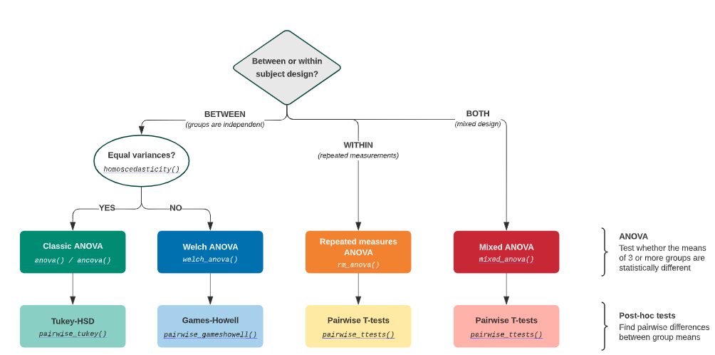

この分析フローに則って分析を進めていきます。

まず、以下のコマンドにより、Pingouinで利用できるデータセットの一覧を確認します。
INPUT:

import pingouin as pg
# 利用可能なデータセット一覧
pg.list_dataset()

OUTPUT:

今回はPingouinパッケージに内包されているanova（生まれつきの髪色と感じる痛みの閾値との関係）データセットを対象に解析していきます。
まず今回使用するデータセットを読み込みます。
INPUT:

df = pg.read_dataset('anova')
df.head()

OUTPUT:

簡単にデータセットの分布を確認します。

sns.barplot(x='Hair color', y='Pain threshold', data=df)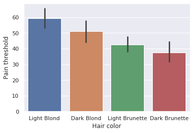

グループ（生まれつきの髪色）ごとに痛みの閾値の平均値が異なることがわかります。
このグループ間の平均値の差が有意かどうかを以降の分析していきます。

今回利用するデータは繰り返しがなくグループ間で独立なので、分析フローの「BETWEEN(groups are independent)」に分岐し、分散の等質性（グループ間の分散:バラツキに差がないこと）を検定します。
INPUT:

# 分散の等質性の検定
pg.homoscedasticity(data=df, dv='Pain threshold', group='Hair color')

OUTPUT:

有意水準を0.05としたとき、pval（p値）が有意水準を上回ります。
したがって、分散が等質であるという帰無仮説を棄却できないので、グループ間の分散が等質であるとみなすことになります。

グループ間の分散が等質な場合、古典的な一元配置分散分析（one-way ANOVA）を実行します。
ちなみに、データに含まれる因子が髪の色の1つだけなので、「一元」配置と呼ばれます。
※もし、グループ間の分散が等質でない場合、一元配置分散分析ではなくウェルチの検定を実行します。
INPUT:

# 一元配置分散分析
pg.anova(data=df, dv='Pain threshold', between='Hair color')

OUTPUT:

p-uncが有意水準0.05を下回るので、2つ以上のグループの標本が同じ平均値を持つ母集団から取られているという帰無仮説が棄却されます。
したがって、グループ間の少なくとも1組は平均値に有意差があるということになります。
ですが、このままだと具体的にどのグループ間の平均値に有意差があるのかがわからないので、さらにTukeyの多重比較によってどのグループ間で差があるのかを確認します。
INPUT:

# Tukeyの多重比較
pg.pairwise_tukey(data=df, dv='Pain threshold', between='Hair color')

OUTPUT:

上の結果から、p値が有意水準0.05を下回る次のグループ間で平均値に有意差があると言えます。

• Dark BlondとDark Brunette
• Dark BrunetteとLight Blond
• Light BlondとLight Brunette

最後に

冒頭でも述べましたが、Pingouinではt値やp値意外の指標も得られるため、簡易に統計解析する場合はPingouinを使った方が良さそうです。（もちろん、深い分析をする際にはRを使うべきですが。）
また、公式ドキュメントを見たところ、Paired plotやBland-Altman plotといった可視化も簡単にできるようです。
データサイエンティストなら知っておいて損はないパッケージだと思います。